Zero knowledge proofs (ZKP) is one of the the most exciting cryptographic inventions since Public-key cryptography. zk-SNARK is a specific type of ZKP which allows one party (the prover) to convince other parties (the verifiers) that the prover faithfully executed a program with some secret information, without conveying any knowledge about the secret information itself. zk-SNARK also generates succinct (hundreds of bytes) proofs that can be verified within the range of miliseconds even though the original computation might be much larger, which means that other than the obvious privacy benefits, zk-SNARK can also be used to trustlessly outsource expensive computation.

To apply zk-SNARK, a computation needs to be expressed in terms of algebraic circuit, converted to a constraint system called R1CS, and then finally a form called “quadratic arithmetic program” (QAP). The intuition of going through this complex transformation is that:

1. A computation can be viewed as series of constraints from the inputs to the outputs, but just expressing a computation in terms of constraints neither make the computation more “succinct” nor make it easier to apply cryptographic algorithms.
2. QAP in a way “compresses” those constraints into one using polynomials, a form which is not only more efficient to verify but also more suitable to apply cryptographic protocols such as Pinocchio or Groth16 to achieve soundness, completeness and zero-knowledgeness.

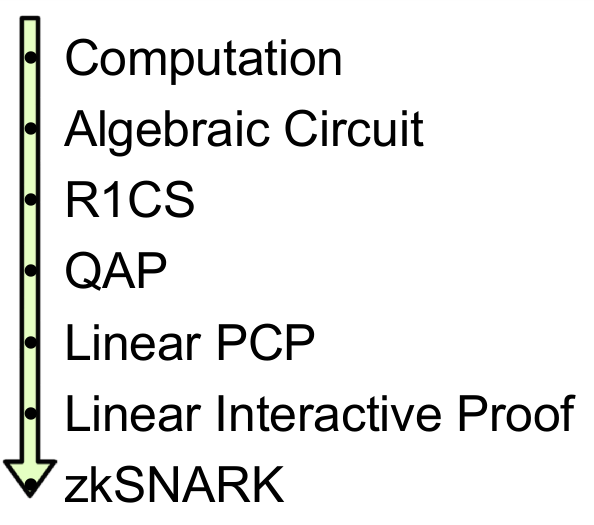
Steps of transformation for zk-SNARK, drawn by Eran Tromer

For more detailed explanations of the QAP transformation, please take a look at Why and How zk-SNARK works by Maksym Petkus or Quadratic Arithmetic Programs: from Zero to Hero by Vitalik Buterin. To use an example in Vitalik’s article, a simple program x³ + x + 5 == 35 can be converted into the following QAP.

QAP for x³ + x + 5 == 35, as in Vitalik’s Quadratic Arithmetic Programs: from Zero to Hero

This article assumes that the readers understand the process of QAP transformation, specifically why proving A(τ)*B(τ)-C(τ) = H(τ)*Z(τ) is important in terms of completenss and soundness. It also assumes some high level understanding of the elliptic curve paring. The purpose of the article is to explain how zk-SNARK works by walking through how it is implemented in Bellman (0.7.0), a rust library used by the first widespread zk-SNARK application ZCash. Bellman currently implements the Groth16 proving system, which can be roughly divided into three parts: Trusted setup, Prover and Verifier. This article discusses each part in details.

Trusted setup

Trusted setup is a process to create what’s called “Common Reference String” (CRS) between provers and verifiers. CRS are basically encrypted secrets that are required by both provers and verifiers to run the cryptographic protocols (e.g. Groth16) in zk-SNARK. Verifiers need to trust that the original secrets (a.k.a toxic waste) are destroyed after the setup process, otherwise the entire proof system breaks down.

First, let’s define some parameters for a computation. We can use m to denote its number of variables, l of which are public. Take x³ + x + 5 = 35 as an example where the solution 3 is the secret. This program can be broken up into the following 3 constraints in the form of A * B = C:

A                  *    B       =      C
———
x                  *    x       =   x_squared
x_squared          *    x       =    x_cubed
(x_cubed + x + 5)  *    1       =     out

There are 4 variables in total (i.e. x, x_squared, x_cubed and out), among which out has a publicly known value of 35. Therefore m and l should be 4 and 1 respectively.

Another important parameter for the computation is the number of constraints n, which determines the target polynomial Z(x). In the above example, the value of n should be 3.

# Target polynomial
Z(x) = (x-1)(x-2)...(x-n)

Assuming that the program is converted to the QAP form, which means that we know the variable polynomials Aᵢ(x), Bᵢ(x) and Cᵢ(x). If the prover knows the value of all variables wᵢ (both the public ones and secret ones), then ultimately (s)he wants to prove the following statement in such a way that reveals nothing about the secret portion of wᵢ:

A(x) * B(x) - C(x) = H(x) * Z(x)
  where
    A(x) = ∑ wᵢAᵢ(x)  -- i in 1..m
    B(x) = ∑ wᵢBᵢ(x)  -- i in 1..m
    C(x) = ∑ wᵢCᵢ(x)  -- i in 1..m

Groth16 protocol is way to achieve that. It requires two paring friendly curves: G1, G2 (with the paring domain GT). During the trusted setup, the first thing it does is to select one random point on each curve: g1 and g2.

Next, it generates the following 5 random field elements: α (alpha), β (beta), γ (gamma), δ (delta) and τ (tau). τ is the secret value at which all the polynomials are evaluated later on. With α and β, it also defines a polynomial Lᵢ(x):

Lᵢ(x) = β * Aᵢ(x) + α * Bᵢ(x) + Cᵢ(x)

With the information created so far, Groth16 generates the following G1 and G2 points (values encrypted using g1 or g2) for the prover:

# G1 elements
α, δ, 1,
τⁱ          # (i in 0..n-1)
Lᵢ(τ)/δ     # (i in l+1..m)
τⁱZ(τ)/δ    # (i in 1..n-2)

# G2 elements
β, δ, 1,
τⁱ          # (i in 0..n-1),

For the verifier, the following points on G1 and G2 are created, along with a pre-computed value g₁ᵅ * g₂ᵝ using elliptic curve paring. Including g₁ᵅ * g₂ᵝ in CRS improves the verification performance since it is needed every time a proof is verified.

# G1 elements
1,
Lᵢ(τ)/γ     # (i in 1..l),

# G2 elements
1, γ, δ

# Gt element
α₁ * β₂

After all these information is created, it is mandatory that random field elements α, β, γ, δ and τ (a.k.a toxic waste) are destroyed. In the Prover and Verifier section, we will discuss how these information is used by both the prover and verifier in such a way that the prover can convince the verifier that A(x) * B(x) - C(x) = H(x) * Z(x) is valid without revealing any secrets. For now let’s take a look at how trusted setup is implemented in Bellman.

Implementation

The code that implements trusted setup in Bellman is located in generator.rs, specifically the generate_random_parameters function. The code that generates g1, g2, α, β, γ, δ and τ is pretty straightforward.

let g1 = E::G1::random(rng);
let g2 = E::G2::random(rng);
let alpha = E::Fr::random(rng);
let beta = E::Fr::random(rng);
let gamma = E::Fr::random(rng);
let delta = E::Fr::random(rng);
let tau = E::Fr::random(rng);

In Bellman, a computation is expressed in “circuits” using the Circuit and ConstraintSystem abstraction. For x³ + x + 5 = 35, which has the following constraints:

x * x = x_squared
x_squared * x = x_cubed
(x_cubed + x + 5) * 1 = out

We can express the 2nd constraint x_squared * x = x_cubed in bellman like this:

// Allocate: x_squared * x = x_cubed
let x_cubed_val = x_squared_val.map(|mut e| {
    e.mul_assign(&x_val.unwrap());
    e
});
let x_cubed = cs.alloc(|| "x_cubed", || {
    x_cubed_val.ok_or(SynthesisError::AssignmentMissing)
})?;
// Enforce: x_squared * x = x_cubed
cs.enforce(
    || "x_cubed",
    |lc| lc + x_squared,
    |lc| lc + x,
    |lc| lc + x_cubed
);

cs in the example above is an instance of a ConstraintSystem. During the trusted setup, circuits are converted to QAP using the KeypairAssembly ConstraintSystem.

/// This is our assembly structure that we'll use to synthesize the
/// circuit into a QAP.
struct KeypairAssembly<Scalar: PrimeField> {
    num_inputs: usize,
    num_aux: usize,
    num_constraints: usize,
    at_inputs: Vec<Vec<(Scalar, usize)>>,
    bt_inputs: Vec<Vec<(Scalar, usize)>>,
    ct_inputs: Vec<Vec<(Scalar, usize)>>,
    at_aux: Vec<Vec<(Scalar, usize)>>,
    bt_aux: Vec<Vec<(Scalar, usize)>>,
    ct_aux: Vec<Vec<(Scalar, usize)>>,
}

When alloc_input or alloc is called to allocate a variable, an empty vector is pushed to at_inputs, bt_inputs, ct_inputs or at_aux, at_aux, at_aux respectively. The index of the empty vector is used to keep track of the newly allocated variables.

These empty vectors is used to store a sequence of (coefficient, constraint_number) tuple for each variable, basically where (which constraint) and how (what coefficient) a particular variable is used in the circuit. enforce function ensures that a sequence of these tuples is stored correctly for each variable.

After the circuit is synthesize with KeypairAssembly (basically all the alloc, alloc_input and enforce in the circuit are executed), what we end up with is essentially the lagrange representation of the public variable polynomials stored in at_inputs, bt_inputs, ct_inputs, and secret variable polynomials in at_aux, bt_aux, ct_aux. We now have Aᵢ(x), Bᵢ(x) and Cᵢ(x)!

Recall that we also need τⁱ (i in 0..n-1) as both G1 and G2 points in the trusted setup. This is called powers of tau, which is important for evaluating polynomials blindly at value τ. Further more, we need τⁱZ(τ)/δ as well where Z(x) is the target polynomial.

This is how powers of tau is calculated in bellman:

let powers_of_tau = powers_of_tau.as_mut();
worker.scope(powers_of_tau.len(), |scope, chunk| {
    for (i, powers_of_tau) in powers_of_tau.chunks_mut(chunk).enumerate() {
        scope.spawn(move |_scope| {
            let mut current_tau_power = tau.pow_vartime(&[(i * chunk) as u64]);

            for p in powers_of_tau {
                p.0 = current_tau_power;
                current_tau_power.mul_assign(&tau);
            }
        });
    }
});

Z(τ)/δ is calculated with

// coeff = Z(x) / δ
let mut coeff = powers_of_tau.z(&tau);
coeff.mul_assign(&delta_inverse);

and coeff is later on multiplied with powers of tau to get τⁱZ(τ)/δ.

The last values we want to create during the trusted setup is Lᵢ(τ)/δ for public variables and Lᵢ(τ)/γ for secret variabes where Lᵢ(x) = β * Aᵢ(x) + α * Bᵢ(x) + Cᵢ(x) as we discussed earlier. Since we already know α, β and Aᵢ(x), Bᵢ(x), Cᵢ(x) at this point, we basically need to evaluate Lᵢ(x) polynomial at the point of τ. This is where powers of tau (τⁱ) comes in handy. Let’s say if Lᵢ(x) is in the form of a*xᵘ+ b*xᵛ + c*xʷ, we just need to find the corresponding τᵘ, τᵛ and τʷ to calculate Lᵢ(τ) = a*τᵘ+ b*τᵛ + c*τʷ. Since i in τⁱ is determined by the number of constraints, we should have all the τⁱ needed for the evaluation.

Here is how Lᵢ(τ)/δ is calculated at τ in Bellman, specifically:

// β * Aᵢ(τ)
at.mul_assign(&beta);
// α * Bᵢ(τ)
bt.mul_assign(&alpha);

// Lᵢ(τ) = β * Aᵢ(τ)
let mut e = at;
// Lᵢ(τ) = β * Aᵢ(τ) + α * Bᵢ(τ)
e.add_assign(&bt);
// Lᵢ(τ) = β * Aᵢ(τ) + α * Bᵢ(τ) + Cᵢ(τ)
e.add_assign(&ct);
// L(τ) / δ  or L(τ) / γ
e.mul_assign(inv);

// g1 ^ (L(τ) / δ) or g1 ^ (L(τ) / γ)
*ext = g1_wnaf.scalar(&e);

As we can see, in order to evaluate Lᵢ(τ), we need to evaluate Aᵢ(τ), Bᵢ(τ) and Cᵢ(τ) as well. If we think about it, Lᵢ(τ), Aᵢ(τ), Bᵢ(τ) and Cᵢ(τ) are the lagrange representation of L(x), A(x), B(x) and C(x). Prover only needs the secret variable portion of the Lᵢ(τ), verifier only needs the public variable portion of the Lᵢ(τ). Here is the VerifyingKey which is created at the end of the trusted setup for the verifier:

let vk = VerifyingKey::<E> {
    // α (G1 element)
    alpha_g1: (g1 * &alpha).to_affine(),
    // β (G2 and G2 elements)
    beta_g1: (g1 * &beta).to_affine(),
    beta_g2: (g2 * &beta).to_affine(),
    // γ (G2 elements)
    gamma_g2: (g2 * &gamma).to_affine(),
    // δ (G1 and G2 elements)
    delta_g1: (g1 * &delta).to_affine(),
    delta_g2: (g2 * &delta).to_affine(),
    // public variable portion of Lᵢ(τ)/γ (G1 element)
    ic,
};

Finally at this point, we have created all the parameters we need, here are all the Parameters that the trusted setup process returns:

Ok(Parameters {
    // VerifyingKey discussed above
    vk,
    // τⁱZ(τ)/δ (G1 element)
    h: Arc::new(h),
    // secret variable portion of Lᵢ(τ)/δ (G1 element)
    l: Arc::new(l),

    // Filter points at infinity away from A/B queries
    // Aᵢ(τ)  (G1 element)
    a: Arc::new(
        a.into_iter()
            .filter(|e| bool::from(!e.is_identity()))
            .collect(),
    ),
    // Bᵢ(τ)  (G1 element)
    b_g1: Arc::new(
        b_g1.into_iter()
            .filter(|e| bool::from(!e.is_identity()))
            .collect(),
    ),
    // Bᵢ(τ)  (G2 element)
    b_g2: Arc::new(
        b_g2.into_iter()
            .filter(|e| bool::from(!e.is_identity()))
            .collect(),
    ),
})

Prover

The prover knows the value of all m variables in the computation, both public input variables (l in total) and secret auxiliary variables (m-l in total). These variables can be represented by wᵢ. When i between 0 to l, wᵢ represents input (public) variables. When i is between l+1 to m, wᵢ represents auxiliary (secret) variables. With this knowledge, the prover wants to construct three values: Aₚ, Bₚ and Cₚ, as defined below:

-- G1 elements
Aₚ = α + A(τ) + r*δ
   where
     A(τ) = ∑ wᵢAᵢ(τ)  -- i in 0..m

-- G2 elements
Bₚ = β + B(τ) + s*δ
   where
     B(τ) = ∑ wᵢBᵢ(τ)  -- i in 0..m

-- G2 elements
Cₚ = L_aux(τ)/δ + H(τ)*(Z(τ)/δ) + s*Aₚ + r*Bₚ - r*s*δ
   where
     -- auxiliary input
     L_aux(τ) = ∑ wᵢLᵢ(τ)  -- i in l+1..m

r and s are randomly generated field elements by the prover.

With Aₚ, Bₚ and Cₚ, the verifier can somehow verify that the statement A(τ)*B(τ) - C(τ) = H(τ)*Z(τ) is valid and therefore confirm that the prover had executed the computation faithfully without revealing the auxiliary variables. We will break down how this is achieved later when we discuss verifiers. For now, let’s focus on how the prover constructs Aₚ, Bₚ and Cₚ.

From the trusted setup, the prover knows the G1 elements α, δ and G2 elements β, δ. The prover also knows the “computation”, which is expressed as R1CS circuit and then converted to Quadratic Arithmetic Program (QAP).

Concretely, the QAP program is expressed using A, B and C where

A(x) = ∑ wᵢAᵢ(x)  -- i in 0..m
B(x) = ∑ wᵢBᵢ(x)  -- i in 0..m
C(x) = ∑ wᵢCᵢ(x)  -- i in 0..m

Also remember that L and H are defined in terms of A, B, C and T, as follows

Lᵢ(x) = β * Aᵢ(x) + α * Bᵢ(x) + Cᵢ(x)
H(x) = (A(x) * B(x) - C(x)) / Z(x)

Knowing the value of all variables wᵢ, the prover has everything needed to construct Aₚ, Bₚ and Cₚ.

Implementation

The prover code in bellman is in located in prover.rs, specifically the create_proof function.

First of all, the circuit is synthesized using the ProvingAssignment data structure, which is also a type of ConstraintSystem.

struct ProvingAssignment<E: Engine> {
    // Density of queries
    a_aux_density: DensityTracker,
    b_input_density: DensityTracker,
    b_aux_density: DensityTracker,

    // Evaluations of A, B, C polynomials
    a: Vec<Scalar<E>>,
    b: Vec<Scalar<E>>,
    c: Vec<Scalar<E>>,

    // Assignments of variables
    input_assignment: Vec<E::Fr>,
    aux_assignment: Vec<E::Fr>,
}

When alloc_input or alloc is called, the actual value of the variable is pushed to input_assignment and aux_assignment vector respectively. Variables are tracked by their position (index) in those vectors.

When enforce is called, it evaluates A, B and C for each operation (in the form of A*B=C) using the variable values in input_assignment and aux_assignment. The evaluation results are pushed to a, b and c vectors respectively. After the entire circuit is synthesized, a, b and c essentially becomes the lagrange representation of A(x), B(x) and C(x).

Aₚ is relatively easy to create, it is equal to α + A(τ) + r*δ (prover:304):

// Aₚ = r*δ
let mut g_a = vk.delta_g1 * &r;
// Aₚ = α + r*δ
AddAssign::<&E::G1Affine>::add_assign(&mut g_a, &vk.alpha_g1);
let mut a_answer = a_inputs.wait()?;
AddAssign::<&E::G1>::add_assign(&mut a_answer, &a_aux.wait()?);
// Aₚ = α + A(τ) + r*δ
AddAssign::<&E::G1>::add_assign(&mut g_a, &a_answer);

Bₚ is computed in a very similiar way. What is more interesting is Cₚ since it involves a more complex H(τ)*(Z(τ)/δ) expression. Recall that H(τ) is basically (A(t) * B(t) - C(t)) / Z(t) and Z(x) is the target polynomial that is publicly known. Here is how H(τ)*(Z(τ)/δ) gets computed (represented by h in the code):

let h = {
    let mut a = EvaluationDomain::from_coeffs(prover.a)?;
    let mut b = EvaluationDomain::from_coeffs(prover.b)?;
    let mut c = EvaluationDomain::from_coeffs(prover.c)?;
    a.ifft(&worker);
    a.coset_fft(&worker);
    b.ifft(&worker);
    b.coset_fft(&worker);
    c.ifft(&worker);
    c.coset_fft(&worker);

    // A * B
    a.mul_assign(&worker, &b);
    drop(b);
    // A * B - C
    a.sub_assign(&worker, &c);
    drop(c);
    // (A * B - C) / Z
    a.divide_by_z_on_coset(&worker);
    a.icoset_fft(&worker);
    let mut a = a.into_coeffs();
    let a_len = a.len() - 1;
    a.truncate(a_len);
    // TODO: parallelize if it's even helpful
    let a = Arc::new(a.into_iter().map(|s| s.0).collect::<Vec<_>>());

    // ((A * B - C) / Z) * (Z / δ)
    multiexp(&worker, params.get_h(a.len())?, FullDensity, a)
};

Now the prover knows H(τ)*(Z(τ)/δ), it becomes a bit easier to computed Cₚ:

let mut g_c;
{
    let mut rs = r;
    rs.mul_assign(&s);

    // Cₚ = r*s*δ
    g_c = vk.delta_g1 * &rs;

    // Cₚ = r*s*δ + s*α
    AddAssign::<&E::G1>::add_assign(&mut g_c, &(vk.alpha_g1 * &s));

    // Cₚ = r*s*δ + s*α + r*β
    AddAssign::<&E::G1>::add_assign(&mut g_c, &(vk.beta_g1 * &r));
}

// Cₚ = s*A(τ) + r*s*δ + s*α + r*β
MulAssign::<E::Fr>::mul_assign(&mut a_answer, s);
AddAssign::<&E::G1>::add_assign(&mut g_c, &a_answer);

// Cₚ = r*B(τ) + s*A(τ) + r*s*δ + s*α + r*β
MulAssign::<E::Fr>::mul_assign(&mut b1_answer, r);
AddAssign::<&E::G1>::add_assign(&mut g_c, &b1_answer);

// Cₚ = H(τ)*(Z(τ)/δ) + r*B(τ) + s*A(τ) + r*s*δ + s*α + r*β
AddAssign::<&E::G1>::add_assign(&mut g_c, &h.wait()?);

// Cₚ = L_aux(τ)/δ + H(τ)*(Z(τ)/δ) + r*B(τ) + s*A(τ) + r*s*δ + s*α + r*β
AddAssign::<&E::G1>::add_assign(&mut g_c, &l.wait()?);

As we can see in the code, Cₚ is actually computed as L_aux(τ)/δ + H(τ)*(Z(τ)/δ) + r*B(τ) + s*A(τ) + r*s*δ + s*α + r*β, which is in fact equivalent to L_aux(τ)/δ + H(τ)*(Z(τ)/δ) + s*Aₚ + r*Bₚ - r*s*δ. Here is why:

# G2 elements
L_aux(τ) = ∑ wᵢLᵢ(τ)  # i in l+1..m. This is the aux input
Cₚ = L_aux(τ)/δ + H(τ)*(Z(τ)/δ) + s*Aₚ + r*Bₚ - r*s*δ
   # Expand Aₚ and Bₚ
   = L_aux(τ)/δ + H(τ)*(Z(τ)/δ) + s*(α + A(τ) + r*δ) + r*(β + B(τ) + s*δ) - r*s*δ
   = L_aux(τ)/δ + H(τ)*(Z(τ)/δ) + s*α + s*A(τ) + r*β + r*B(τ) + r*s*δ

At this point, Aₚ, Bₚ and Cₚ are computed and prover completes the proof.

Ok(Proof {
    // Aₚ
    a: g_a.to_affine(),
    // Bₚ
    b: g_b.to_affine(),
    // Cₚ
    c: g_c.to_affine(),
})

Verifier

The goal of the verifier is to take the proof from the prover, i.e. Aₚ, Bₚ and Cₚ, and verify that the following equation holds:

Aₚ*Bₚ = α*β + (L_input(τ)/γ)*γ + Cₚ*δ
  where
    -- input (public) variables
    L_input(τ) = ∑ wᵢLᵢ(τ) -- i in 0..l

To see what exactly does it mean if this equation holds, we can try to expand on both the left hand side (LHS) and the right hand side (RHS) of the equation.

LHS

Aₚ*Bₚ is equivalent to A(τ)*B(τ) + REM:

Aₚ*Bₚ = A(τ)*B(τ) + REM
  where
    REM = α*β + α*B(τ) + β*A(τ) + α*s*δ + s*δ*A(τ) + r*δ*B(τ) + r*β*δ + r*s*δ*δ

Aₚ*Bₚ
# Expand Aₚ = (α + A(τ) + r*δ)
# Expand Bₚ = (β + B(τ) + s*δ)
= (α + A(τ) + r*δ) * (β + B(τ) + s*δ)
= α*β + α*B(τ) + α*s*δ + β*A(τ) + A(τ)*B(τ) + s*δ*A(τ) + r*β*δ + r*δ*B(τ) + r*s*δ*δ
= A(τ)*B(τ) + α*β + α*B(τ) + β*A(τ) + α*s*δ + s*δ*A(τ) + r*δ*B(τ) + r*β*δ + r*s*δ*δ
# Let REM = α*β + α*B(τ) + β*A(τ) + α*s*δ + s*δ*A(τ) + r*δ*B(τ) + r*β*δ + r*s*δ*δ
= A(τ)*B(τ) + REM

RHS

α*β + (L_input/γ)*γ + Cₚ*δ is equivalent to C(τ) + H(τ)*Z(τ) + REM:

α*β + (L_input/y)*y + Cₚ*δ = C(τ) + H(τ)*Z(τ) + REM
  where
    REM = α*β + α*B(τ) + β*A(τ) + α*s*δ + s*δ*A(τ) + r*δ*B(τ) + r*β*δ + r*s*δ*δ

α*β + (L_input/γ)*γ + Cₚ*δ
# expand Cₚ = L_aux/δ + H(τ)*(Z(τ)/δ) + s*Aₚ + r*Bₚ - r*s*δ
= α*β + L_input(τ) + (L_aux(τ)/δ + H(τ)*(Z(τ)/δ) + s*Aₚ + r*Bₚ - r*s*δ)*δ
= α*β + L_input(τ) + L_aux(τ) + H(τ)*Z(τ) + s*δ*Aₚ + r*δ*Bₚ - r*s*δ*δ
# L(τ) = L_input(τ) + L_aux(τ)
= α*β + L(τ) + H(τ)*Z(τ) + s*δ*Aₚ + r*δ*Bₚ - r*s*δ*δ
# expand Aₚ = α + A(τ) + r*δ
# expand Bₚ = β + B(τ) + s*δ
= α*β + L(τ) + H(τ)*Z(τ) + s*δ*(α + A(τ) + r*δ) + r*δ*(β + B(τ) + s*δ) - r*s*δ*δ
= α*β + L(τ) + H(τ)*Z(τ) + α*s*δ + s*δ*A(τ) + r*s*δ*δ + r*β*δ + r*δ*B(τ)
# expand L(τ) = α*B(τ) + β*A(τ) + C(τ)
= α*β + α*B(τ) + β*A(τ) + C(τ) + H(τ)*Z(τ) + α*s*δ + s*δ*A(τ) + r*s*δ*δ + r*β*δ + r*δ*B(τ)
= C(τ) + H(τ)*Z(τ) + α*β + α*B(τ) + β*A(τ) + α*s*δ + s*δ*A(τ) + r*δ*B(τ) + r*β*δ + r*s*δ*δ
# Let REM = α*β + α*B(τ) + β*A(τ) + α*s*δ + s*δ*A(τ) + r*δ*B(τ) + r*β*δ + r*s*δ*δ
= C(τ) + H(τ)*Z(τ) + REM

If we can prove LHS = RHS, then after removing REM on both sides, we also proved that A(τ)*B(τ)-C(τ) = H(τ)*Z(τ), which is the end goal of the verifier! Once this is valid, the verifier is confident that the program is executed faithfully with correct values of the auxiliary variables.

Implementation

The verification code in Bellman is located at verifier.rs. As explained by the comments, the original equation Aₚ*Bₚ = α*β + (L_input(τ)/γ)*γ + Cₚ*δ is converted to Aₚ*Bₚ + (L_input(τ)/γ)*(-γ) + Cₚ*(-δ) = α*β, which only requires one final exponentiation (verifier.rs:44).

// Code that proves:
// Aₚ*Bₚ + (L_input(τ)/γ)*(-γ) + Cₚ*(-δ) = α*β

Ok(E::final_exponentiation(&E::miller_loop(
    [
        // Aₚ*Bₚ
        (&proof.a.prepare(), &proof.b.prepare()),
        // (L_input(τ)/γ)*(-γ)
        (&acc.into_affine().prepare(), &pvk.neg_gamma_g2),
        // Cₚ*(-δ)
        (&proof.c.prepare(), &pvk.neg_delta_g2),
    ]
    .iter(),
))
.unwrap()
    // α*β
    == pvk.alpha_g1_beta_g2)

The E::final_exponentiation and E::miller_loop functions are two steps needed to compute the elliptic curve paring. The paring of α*β (pvk.alpha_g1_beta_g2) is already pre-computed in the setup phase.

Summary

In this article, we walked through how zk-SNARK with Groth16 protocol is implemented in Bellman, which actually powers a nearly 1 billion dollar cryptocurrency (at the time of writing). Instead of just relying on government regulations and the mercy of big internet companies, I hope zk-SNARK and ZKP in general can be part of the solution for our privacy issues in the future.

References

1. Quadratic Arithmetic Programs: from Zero to Hero
2. Exploring Elliptic Curve Pairings
3. Zk-SNARKs: Under the Hood
4. Why and How zk-SNARK Works
5. Paring in Cryptography
6. Groth16
7. Bellman: zk-SNARKs in Rust